These notes are based on the tutorial I gave at the Geometric Methods in Optimization and Sampling Boot Camp at the Simons Institute in Berkeley.
Suppose we wish to obtain samples from some probability measure  on
on  . If has a sufficiently well-behaved density
  with respect to the Lebesgue measure, i.e.,
 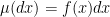 , then we can use the (overdamped) continuous-time Langevin dynamics, governed by the Ito stochastic differential equation (SDE)
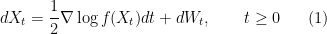
where the initial condition  is generated according to some probability law
  , and
, and  is the standard
  -dimensional Brownian motion. Let
  denote the probability law of
  . Then, under appropriate regularity conditions on , one can establish the following:
In this sense, the Langevin process (1) gives only approximate samples from . I would like to discuss an alternative approach that uses diffusion processes to obtain exact samples in finite time. This approach is based on ideas that appeared in two papers from the 1930s by Erwin Schrödinger in the context of physics, and is now referred to as the Schrödinger bridge problem.
We will now assume that the target probability measure has a density with respect to the canonical Gaussian measure on , i.e.,

We will also assume that is everywhere strictly positive. Our goal is to construct an Ito process governed by the SDE
![\displaystyle dX_t = b(X_t,t)dt + dW_t, \qquad t \in [0,1] \ \ \ \ \ (2)](https://s0.wp.com/latex.php?latex=%5Cdisplaystyle++%09dX_t+%3D+b%28X_t%2Ct%29dt+%2B+dW_t%2C+%5Cqquad+t+%5Cin+%5B0%2C1%5D+%5C+%5C+%5C+%5C+%5C+%282%29&bg=ffffff&fg=000000&s=0&c=20201002)
starting at  , such that:
-
 has probability law ;
-
 , the probability law of the process
 ![{(X_t)_{t \in [0,1]}}](https://s0.wp.com/latex.php?latex=%7B%28X_t%29_%7Bt+%5Cin+%5B0%2C1%5D%7D%7D&bg=ffffff&fg=000000&s=0&c=20201002) , is optimal in the sense that, among all the diffusion processes with values in starting at the origin at
, is optimal in the sense that, among all the diffusion processes with values in starting at the origin at  and having the marginal distribution at
  , it remains “as close as possible” to the standard Brownian motion in the sense to be made precise below.
Note that the drift in (2) is time-dependent. This problem has been studied from many angles, and the optimal drift has an explicit form. My goal here is to give what is, to the best of my knowledge, a somewhat new and rather transparent derivation of the solution to the Schrödinger bridge problem. The main idea is based on a rather neat trick that I picked up from a paper by Hiroshi Ezawa, John Klauder, and Larry Shepp (although it was already present in some form in an earlier short paper by Václav Beneš and Shepp). The presentation will be rather informal, but every step can be made rigorous.
1. The Schrödinger bridge problem
The basic problem can be stated as follows. Let  denote the space of continuous functions (paths) from
 ![{[0,1]}](https://s0.wp.com/latex.php?latex=%7B%5B0%2C1%5D%7D&bg=ffffff&fg=000000&s=0&c=20201002) into , and let
into , and let ![{W = (W_t)_{t \in [0,1]}}](https://s0.wp.com/latex.php?latex=%7BW+%3D+%28W_t%29_%7Bt+%5Cin+%5B0%2C1%5D%7D%7D&bg=ffffff&fg=000000&s=0&c=20201002) denote the canonical coordinate process on : For any
denote the canonical coordinate process on : For any  ,
,  . Let
. Let  denote the Wiener measure on , under which
  is the standard -dimensional Brownian motion on . Given any probability measure on , we will denote by
  the marginal probability law of the value of the path at time
  . With this, we consider the set

where  denotes the Dirac probability measure on centered at the origin. Our goal is to find

where  denotes the relative entropy between two probability measures on . We will need to do two things: (a) show that
  exists and is unique, and (b) show that it is the probability law of a diffusion process governed by an Ito SDE of the form (2).
To take care of (a), all we need is the chain rule for the relative entropy. Fix an arbitrary  ; without loss of generality, we can assume that is absolutely continuous with respect to the Wiener measure , i.e.,
  . The chain rule then gives

where  (respectively,
  ) denotes the conditional probability law of
 ![{X = (X_t)_{t \in [0,1]}}](https://s0.wp.com/latex.php?latex=%7BX+%3D+%28X_t%29_%7Bt+%5Cin+%5B0%2C1%5D%7D%7D&bg=ffffff&fg=000000&s=0&c=20201002) given
given  under (respectively, ). The conditional probability measure is well-known, and gives the probability law of the Brownian bridge process, i.e., the standard Brownian motion pinned to the point
  at . Now, since , we have
  , whereas
  for the Wiener measure . Thus, we have the following for the right-hand side of (3):

where equality holds if and only if  almost everywhere. This immediately implies two things:
From (4), it is easy to obtain an explicit expression for the Radon–Nikodym derivative  : Let
: Let  be an arbitrary bounded measurable real-valued function on . Then, using the fact that
  , (4), and the law of iterated expectation, we can write
![\displaystyle \begin{array}{rcl} {\mathbb E}_{Q^\mu}[F(X)] &=& {\mathbb E}_\mu[{\mathbb E}_{Q^\mu}[F(X)|X_1]] \\ &=& {\mathbb E}_\mu[{\mathbb E}_P[F(X)|X_1]] \\ &=& {\mathbb E}_\gamma[f(X_1){\mathbb E}_P[F(X)|X_1]] \\ &=& {\mathbb E}_\gamma[E_P[f(X_1)F(X)|X_1]] \\ &=& {\mathbb E}_P[f(W_1)F(W)], \end{array}](https://s0.wp.com/latex.php?latex=%5Cdisplaystyle++%5Cbegin%7Barray%7D%7Brcl%7D++%09%7B%5Cmathbb+E%7D_%7BQ%5E%5Cmu%7D%5BF%28X%29%5D+%26%3D%26+%7B%5Cmathbb+E%7D_%5Cmu%5B%7B%5Cmathbb+E%7D_%7BQ%5E%5Cmu%7D%5BF%28X%29%7CX_1%5D%5D+%5C%5C+%09%26%3D%26+%7B%5Cmathbb+E%7D_%5Cmu%5B%7B%5Cmathbb+E%7D_P%5BF%28X%29%7CX_1%5D%5D+%5C%5C+%09%26%3D%26+%7B%5Cmathbb+E%7D_%5Cgamma%5Bf%28X_1%29%7B%5Cmathbb+E%7D_P%5BF%28X%29%7CX_1%5D%5D+%5C%5C+%09%26%3D%26+%7B%5Cmathbb+E%7D_%5Cgamma%5BE_P%5Bf%28X_1%29F%28X%29%7CX_1%5D%5D+%5C%5C+%09%26%3D%26+%7B%5Cmathbb+E%7D_P%5Bf%28W_1%29F%28W%29%5D%2C+%5Cend%7Barray%7D+&bg=ffffff&fg=000000&s=0&c=20201002)
where the first equation is due to the fact that  , in the second equation we have used the fact that the conditional laws
 ![{Q^\mu[\cdot|X_1 = x]}](https://s0.wp.com/latex.php?latex=%7BQ%5E%5Cmu%5B%5Ccdot%7CX_1+%3D+x%5D%7D&bg=ffffff&fg=000000&s=0&c=20201002) and
and ![{P[\cdot|X_1 = x]}](https://s0.wp.com/latex.php?latex=%7BP%5B%5Ccdot%7CX_1+%3D+x%5D%7D&bg=ffffff&fg=000000&s=0&c=20201002) coincide, and in the last equation denotes the standard Brownian motion process with process law . That is, the Radon–Nikodym derivative of with respect to , as a function of the path , depends only on the terminal point
coincide, and in the last equation denotes the standard Brownian motion process with process law . That is, the Radon–Nikodym derivative of with respect to , as a function of the path , depends only on the terminal point  and takes the form

where, as we recall, denotes the density of the target measure with respect to the standard Gaussian measure  on . Thus, the optimal measure is simply the law of the standard -dimensional Brownian motion on , “conditioned” to have law at .
2. The gradient ansatz and the Girsanov transformation
In principle, (5) already tells us that we can obtain samples from by “reweighting” the Brownian paths using the weight factor  that depends only on . What we are after, however, is something different: Instead of reweighting, we would like to construct a “transport” map
  such that
  , i.e., the optimal measure is the pushforward of the Wiener measure by
  :
:
![\displaystyle {\mathbb E}_{Q^\mu}[F(X)] = {\mathbb E}_P[F\circ T(W)]](https://s0.wp.com/latex.php?latex=%5Cdisplaystyle++%09%7B%5Cmathbb+E%7D_%7BQ%5E%5Cmu%7D%5BF%28X%29%5D+%3D+%7B%5Cmathbb+E%7D_P%5BF%5Ccirc+T%28W%29%5D+&bg=ffffff&fg=000000&s=0&c=20201002)
for any bounded measurable  . Moreover, we want this to be such that the “transported” process
  is an Ito diffusion process. In order to construct such a map, we will use a fundamental result in stochastic calculus, the Girsanov theorem, which gives the necessary and sufficient condition for a probability measure on to be absolutely continuous with respect to the Wiener measure .
In order to make use of it, we will first make the gradient ansatz, i.e., we will assume that the diffusion process we seek is governed by an Ito SDE of the form
![\displaystyle dX_t = -\nabla v(X_t,t)dt + dW_t, \qquad X_0 = 0, t \in [0,1] \ \ \ \ \ (6)](https://s0.wp.com/latex.php?latex=%5Cdisplaystyle++%09dX_t+%3D+-%5Cnabla+v%28X_t%2Ct%29dt+%2B+dW_t%2C+%5Cqquad+X_0+%3D+0%2C+t+%5Cin+%5B0%2C1%5D+%5C+%5C+%5C+%5C+%5C+%286%29&bg=ffffff&fg=000000&s=0&c=20201002)
where  denotes the gradient with respect to the space variable. Then we will show that we can choose a suitable function
 ![{v : {\mathbb R}^d \times [0,1] \rightarrow {\mathbb R}}](https://s0.wp.com/latex.php?latex=%7Bv+%3A+%7B%5Cmathbb+R%7D%5Ed+%5Ctimes+%5B0%2C1%5D+%5Crightarrow+%7B%5Cmathbb+R%7D%7D&bg=ffffff&fg=000000&s=0&c=20201002) which is twice continuously differentiable in and once continuously differentiable in , such that the probablity law of the resulting process
which is twice continuously differentiable in and once continuously differentiable in , such that the probablity law of the resulting process  will be given by . To motivate the introduction of the gradient ansatz, it is useful to compare the SDE (6) with the Langevin SDE (1) — the latter has a time-invariant drift given by the gradient of the log-density of with respect to the Lebesgue measure, while in the former we are using a time-varying drift since our goal is to obtain a sample from at time , and intuition suggests that a nonstationary process is needed to make this work.
At any rate, denoting by the probability law of the process (6), we can use the Girsanov theorem to write down the Radon–Nikodym derivative of with respect to :

Comparing (7) with (5), the path forward is now clear: We need to show that  can be chosen in such a way that the right-hand side of (7) is equal to . This is where the Ezawa–Klauder–Shepp trick comes in. The key idea is to eliminate the Ito integral in (7) and then to reduce the problem to solving a suitable partial differential equation (PDE).
Let us define the process ![{(V_t)_{t \in [0,1]}}](https://s0.wp.com/latex.php?latex=%7B%28V_t%29_%7Bt+%5Cin+%5B0%2C1%5D%7D%7D&bg=ffffff&fg=000000&s=0&c=20201002) by
by  . Ito’s lemma then gives

where  is the Laplacian. Integrating and rearranging, we obtain

Substituting this into (7) and using the definition of  gives
gives

If we are to have any hope of reducing the right-hand side to an expression that depends only on , we need to ensure that the integral over is identically zero.
3. The PDE connection
One way of guaranteeing this is to assume that solves the PDE
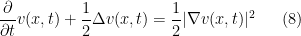
for all ![{(x,t) \in {\mathbb R}^d \times [0,1]}](https://s0.wp.com/latex.php?latex=%7B%28x%2Ct%29+%5Cin+%7B%5Cmathbb+R%7D%5Ed+%5Ctimes+%5B0%2C1%5D%7D&bg=ffffff&fg=000000&s=0&c=20201002) , subject to the terminal condition
, subject to the terminal condition 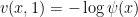 for some strictly positive function
  to be chosen later. Assuming that such a exists, we will then have

which means that  should be chosen in such a way that
  for all
  . Now, the PDE (8) is nonlinear in due to the presence of the squared norm of the gradient of on the right-hand side. However, it is known from the theory of PDEs that we can convert it into a linear PDE that can be solved explicitly; this is accomplished by making the logarithmic (or Cole–Hopf) transformation
  . It is then a straightforward if tedious exercise in multivariate calculus to show that the function
  solves a much nicer linear PDE
on ![{{\mathbb R}^d \times [0,1]}](https://s0.wp.com/latex.php?latex=%7B%7B%5Cmathbb+R%7D%5Ed+%5Ctimes+%5B0%2C1%5D%7D&bg=ffffff&fg=000000&s=0&c=20201002) subject to the terminal condition
subject to the terminal condition  . The solution of (10) is given by the Feynman–Kac formula, one of the remarkable connections between the theory of (parabolic) PDEs and diffusion processes: For any and
 ![{t \in [0,1]}](https://s0.wp.com/latex.php?latex=%7Bt+%5Cin+%5B0%2C1%5D%7D&bg=ffffff&fg=000000&s=0&c=20201002) ,
,
![\displaystyle h(x,t) = {\mathbb E}_P[\psi(W_1)|W_t = x]. \ \ \ \ \ (11)](https://s0.wp.com/latex.php?latex=%5Cdisplaystyle++%09h%28x%2Ct%29+%3D+%7B%5Cmathbb+E%7D_P%5B%5Cpsi%28W_1%29%7CW_t+%3D+x%5D.+%5C+%5C+%5C+%5C+%5C+%2811%29&bg=ffffff&fg=000000&s=0&c=20201002)
The proof of (11) is a simple application of Ito’s lemma: for any ,

Taking the conditional expectation given  and using the fact that solves (10), we obtain (11).
Going back to (8), we can now write
![\displaystyle v(x,t) = - \log h(x,t) = - \log {\mathbb E}_P[\psi(W_1)|W_t = x],](https://s0.wp.com/latex.php?latex=%5Cdisplaystyle++%09v%28x%2Ct%29+%3D+-+%5Clog+h%28x%2Ct%29+%3D+-+%5Clog+%7B%5Cmathbb+E%7D_P%5B%5Cpsi%28W_1%29%7CW_t+%3D+x%5D%2C+&bg=ffffff&fg=000000&s=0&c=20201002)
and, in particular, ![{v(0,0) = - \log {\mathbb E}_P[\psi(W_1)|W_0 = 0] = -\log {\mathbb E}_P[\psi(W_1)] = - \log {\mathbb E}_\gamma[\psi]}](https://s0.wp.com/latex.php?latex=%7Bv%280%2C0%29+%3D+-+%5Clog+%7B%5Cmathbb+E%7D_P%5B%5Cpsi%28W_1%29%7CW_0+%3D+0%5D+%3D+-%5Clog+%7B%5Cmathbb+E%7D_P%5B%5Cpsi%28W_1%29%5D+%3D+-+%5Clog+%7B%5Cmathbb+E%7D_%5Cgamma%5B%5Cpsi%5D%7D&bg=ffffff&fg=000000&s=0&c=20201002) . Substituting all of this into (9) gives
. Substituting all of this into (9) gives
![\displaystyle \frac{dQ}{dP}(W) = \frac{h(W_1,1)}{h(0,0)} = \frac{\psi(W_1)}{{\mathbb E}_\gamma[\psi]},](https://s0.wp.com/latex.php?latex=%5Cdisplaystyle++%09%5Cfrac%7BdQ%7D%7BdP%7D%28W%29+%3D+%5Cfrac%7Bh%28W_1%2C1%29%7D%7Bh%280%2C0%29%7D+%3D+%5Cfrac%7B%5Cpsi%28W_1%29%7D%7B%7B%5Cmathbb+E%7D_%5Cgamma%5B%5Cpsi%5D%7D%2C+&bg=ffffff&fg=000000&s=0&c=20201002)
which means that we should evidently choose  so that
  . Moreover, using the known Gaussian form of the transition probability densities of the Brownian motion, we can give the drift in (6) explicitly as
![\displaystyle \begin{array}{rcl} -\nabla v(x,t) &=& \nabla \log {\mathbb E}_\gamma[f(x + \sqrt{1-t}Z)] \\ &=& \nabla \log \int_{{\mathbb R}^d} f(x + \sqrt{1-t}z) e^{-|z|^2/2} dz \end{array}](https://s0.wp.com/latex.php?latex=%5Cdisplaystyle++%5Cbegin%7Barray%7D%7Brcl%7D++%09-%5Cnabla+v%28x%2Ct%29+%26%3D%26+%5Cnabla+%5Clog+%7B%5Cmathbb+E%7D_%5Cgamma%5Bf%28x+%2B+%5Csqrt%7B1-t%7DZ%29%5D+%5C%5C+%09%26%3D%26+%5Cnabla+%5Clog+%5Cint_%7B%7B%5Cmathbb+R%7D%5Ed%7D+f%28x+%2B+%5Csqrt%7B1-t%7Dz%29+e%5E%7B-%7Cz%7C%5E2%2F2%7D+dz+%5Cend%7Barray%7D+&bg=ffffff&fg=000000&s=0&c=20201002)
where  is distributed according to the canonical Gaussian measure . This is known as the Föllmer drift (see this paper by Ronen Eldan and James Lee for more information and for further references).
4. The optimal control formulation
Those of you who are familiar with the theory of controlled diffusion processes should recognize the PDE (8) as the Hamilton–Jacobi–Bellman equation for the value function of a certain finite-horizon optimal stochastic control problem. While I do not want to get too much into details, I will sketch the basic idea. The first step is to use the identity

where the minimum is achieved uniquely by  , to rewrite (8) in the equivalent form

for with  . The stochastic control connection is as follows: We seek an adapted control process
 ![{u = (u_t)_{t \in [0,1]}}](https://s0.wp.com/latex.php?latex=%7Bu+%3D+%28u_t%29_%7Bt+%5Cin+%5B0%2C1%5D%7D%7D&bg=ffffff&fg=000000&s=0&c=20201002) to minimize the expected cost
to minimize the expected cost
![\displaystyle J(u) := {\mathbb E}^u \left[ \frac{1}{2}\int^1_0 |u_t|^2 dt - \log f(X^u_1) \right], \ \ \ \ \ (13)](https://s0.wp.com/latex.php?latex=%5Cdisplaystyle++%09J%28u%29+%3A%3D+%7B%5Cmathbb+E%7D%5Eu+%5Cleft%5B+%5Cfrac%7B1%7D%7B2%7D%5Cint%5E1_0+%7Cu_t%7C%5E2+dt+-+%5Clog+f%28X%5Eu_1%29+%5Cright%5D%2C+%5C+%5C+%5C+%5C+%5C+%2813%29&bg=ffffff&fg=000000&s=0&c=20201002)
where ![{{\mathbb E}^u[\cdot]}](https://s0.wp.com/latex.php?latex=%7B%7B%5Cmathbb+E%7D%5Eu%5B%5Ccdot%5D%7D&bg=ffffff&fg=000000&s=0&c=20201002) denotes expectation with respect to the controlled diffusion process
denotes expectation with respect to the controlled diffusion process
![\displaystyle dX^u_t = u_t dt + dW_t, \qquad X^u_0 = 0, t \in [0,1]. \ \ \ \ \ (14)](https://s0.wp.com/latex.php?latex=%5Cdisplaystyle++%09dX%5Eu_t+%3D+u_t+dt+%2B+dW_t%2C+%5Cqquad+X%5Eu_0+%3D+0%2C+t+%5Cin+%5B0%2C1%5D.+%5C+%5C+%5C+%5C+%5C+%2814%29&bg=ffffff&fg=000000&s=0&c=20201002)
Here, the integral  is the control cost, while
  is the terminal cost at . It can then be shown using the so-called verification theorem in the theory of controlled diffusions that the solution
  of the PDE (12) gives the value function (or the optimal cost-to-go function)
![\displaystyle v(x,t) := \min_{u} {\mathbb E}^u \Bigg[\frac{1}{2}\int^1_t |u_s|^2 ds - \log f(X^u_1) \Bigg|X^u_t = x\Bigg],](https://s0.wp.com/latex.php?latex=%5Cdisplaystyle++%09v%28x%2Ct%29+%3A%3D+%5Cmin_%7Bu%7D+%7B%5Cmathbb+E%7D%5Eu+%5CBigg%5B%5Cfrac%7B1%7D%7B2%7D%5Cint%5E1_t+%7Cu_s%7C%5E2+ds+-+%5Clog+f%28X%5Eu_1%29+%5CBigg%7CX%5Eu_t+%3D+x%5CBigg%5D%2C+&bg=ffffff&fg=000000&s=0&c=20201002)
so that, in particular,  . Here, the idea is that we add the drift
  to the standard Brownian motion to steer the process towards the target distribution at , while keeping the total “control effort” small. Of course, from the preceding derivations we know that
 ![{v(0,0) = - \log {\mathbb E}_\gamma[f(Z)] = 0}](https://s0.wp.com/latex.php?latex=%7Bv%280%2C0%29+%3D+-+%5Clog+%7B%5Cmathbb+E%7D_%5Cgamma%5Bf%28Z%29%5D+%3D+0%7D&bg=ffffff&fg=000000&s=0&c=20201002) , and that the optimal control is of the state feedback form, given explicitly by the Föllmer drift. Moreover, one can show using the Girsanov theorem that every can be realized as a controlled process of the form (14) for some admissible drift , so that
, and that the optimal control is of the state feedback form, given explicitly by the Föllmer drift. Moreover, one can show using the Girsanov theorem that every can be realized as a controlled process of the form (14) for some admissible drift , so that  has law and
![\displaystyle D(Q \| P) = {\mathbb E}^u \left[ \frac{1}{2}\int^1_0 |u_t|^2 dt \right] = J(u) + {\mathbb E}^u[\log f(X^u_1)] = J(u) + D(\mu \| \gamma).](https://s0.wp.com/latex.php?latex=%5Cdisplaystyle++%09D%28Q+%5C%7C+P%29+%3D+%7B%5Cmathbb+E%7D%5Eu+%5Cleft%5B+%5Cfrac%7B1%7D%7B2%7D%5Cint%5E1_0+%7Cu_t%7C%5E2+dt+%5Cright%5D+%3D+J%28u%29+%2B+%7B%5Cmathbb+E%7D%5Eu%5B%5Clog+f%28X%5Eu_1%29%5D+%3D+J%28u%29+%2B+D%28%5Cmu+%5C%7C+%5Cgamma%29.+&bg=ffffff&fg=000000&s=0&c=20201002)
This implies, in turn, that the Föllmer drift that gives the optimal measure is the most efficient control, in the sense that the sum of the expected control cost and the expected terminal cost is identically zero, and therefore none of the control effort is wasted along the way. Of course, one could have started with this optimal control formulation (as I do in this paper with Belinda Tzen), but I feel that the above derivation is more “elementary” in the sense that it does not rely on any specialized knowledge beyond basic stochastic calculus.
, then
for all
— in fact, it is often possible to show that there exists a constant
that depends only on

;

Welcome back! It’s been a long break.