Stochastic kernels vs. conditional probability distributions

Larry Wasserman‘s recent post about misinterpretation of p-values is a good reminder about a fundamental distinction anyone working in information theory, control or machine learning should be aware of — namely, the distinction between stochastic kernels and conditional probability distributions.

Roughly speaking, stochastic kernels are building blocks, objects that have to be interconnected in order to instantiate stochastic systems. Conditional probability distributions, on the other hand, arise only when we apply Bayes’ theorem to joint probability distributions induced by these interconnections.

At a very high level of abstraction, we may imagine a space of observations or outcomes ${{\mathsf Y}}$ and a space of states or inputs ${{\mathsf X}}$ . Each possible state ${x \in {\mathsf X}}$ induces a probability distribution over ${{\mathsf Y}}$ — let’s denote it by ${P_x}$ . The interpretation is that if the state is ${x}$ , then the probability that we observe an outcome in some set ${A \subseteq {\mathsf Y}}$ is ${P_x(A)}$ . Notice that this stipulation has the flavor of a conditional statement: if A then B. Mathematical statisticians (going back to Abraham Wald, and greatly elaborated by Lucien Le Cam and his followers) like to think of the collection ${(P_x : x\in{\mathsf X})}$ as an experiment that reveals something about the state in ${{\mathsf X}}$ through a random observation in ${{\mathsf Y}}$ . Note that ${(P_x : x \in {\mathsf X})}$ is not a set of probability distributions — two distinct ${x}$ ‘s may carry two identical ${P_x}$ ‘s (which would indicate that these two ${x}$ ‘s are statistically indistinguishable on the basis of observations); or, in the simplest case of a binary state space ${{\mathsf X}=\{0,1\}}$ , the experiment that has ${P_0 = P}$ and ${P_1 = Q}$ is different from the one with ${P_0 = Q}$ and ${P_1 = P}$ , where ${P}$ and ${Q}$ are two fixed probability distributions on ${{\mathsf Y}}$ . So perhaps it is better to think about the experiment ${(P_x)}$ as a function from ${{\mathsf X}}$ into ${{\mathcal P}({\mathsf Y})}$ , the space of all probability distributions on ${{\mathsf Y}}$ . When we impose a measurable structure on the state space ${{\mathsf X}}$ as well and then require this function to be sufficiently well-behaved, so that the mapping ${x \mapsto P_x(A)}$ is nice (read: measurable) for any ${A}$ , then we have a stochastic kernel.

Larry’s point about p-values is as follows: a binary hypothesis testing problem is a binary experiment ${(P_0,P_1)}$ , where ${P_0}$ and ${P_1}$ can be thought of as two fixed distributions on some observation space ${{\mathsf Y}}$ that “explain” the observed outcomes given each hypothesis. If we compute a test statistic ${Z : {\mathsf Y} \rightarrow {\mathbb R}}$ and let ${z}$ be the realized value of ${Z}$ , then the p-value (for a two-sided test) is

$\displaystyle p = P_0\left(\{ y \in {\mathsf Y}: |Z(y)| > |z|\}\right).$

It’s not a conditional probability of anything, but rather the probability a certain event would have if the state were ${0}$ . In order to have conditioning, all relevant quantities must be instantiated as random variables. Let’s consider an example any information theorist should relate to: a binary symmetric channel.

The ingredients are: the input space ${{\mathsf X} = \{0,1\}}$ , the output space ${{\mathsf Y} = \{0,1\}}$ , and the experiment

$\displaystyle P_0 = {\rm Bernoulli}(p), \qquad P_1 = {\rm Bernoulli}(1-p),$

where ${p \in [0,1]}$ is the channel’s crossover probability. We often write the channel transition probabilities suggestively as ${P_{Y|X}(0|0)}$ etc., but that is, strictly speaking, incorrect. Until we specify something about the input to the channel, all we have is the experiment ${(P_0,P_1)}$ , together with a list of possible statements like

if the input is ${0}$ , then the probability of observing ${0}$ at the output is ${1-p}$

and the like. If we now say that the input is a random variable ${X}$ taking values in ${{\mathsf X}}$ according to a given distribution 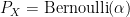${P_X = {\rm Bernoulli}(\alpha)}$ , then we may make conditional probability statements and compute conditional probability distributions ${P_{Y|X}}$ and ${P_{X|Y}}$ . Of course, in this case it so happens that the conditional probability distribution ${P_{Y|X}}$ is already given in terms of the original experiment. But, properly speaking, this conditional object does not exist until we fix ${P_X}$ . Even more dramatically, the posterior ${P_{X|Y}}$ does not exist at all until we specify ${P_X}$ , interconnect the source of ${X}$ to the kernel corresponding to the experiment ${(P_0,P_1)}$ , and start doing what Bayesians would call inverse inference. This distinction between kernel specifications and conditional probability distributions may seem purely notational, but it matters a great deal as soon as feedback enters into the picture.

The clearest statement on the implications of this distinction has been made by Hans Witsenhausen in his influential paper on separation between estimation and control:

When the control laws have been selected and instrumented, and only then, the control variables (and the state and output variables, and the cost) become random variables, that is, become functionally related to the given random variables (noise, initial state) and therefore become functionally related to the underlying probability space. But to the designer who is still seeking for good control laws and has not made a selection yet, the realizations of control are not even random variables. They are just “random variables to be” of yet uncertain status.

I also recommend a recent paper by Jan Willems on what he terms “open stochastic systems.” It is best to illustrate the main idea of this paper through another example any information theorist should be familiar with: additive white Gaussian noise (AWGN) channel. We are all used to writing it down as

$\displaystyle Y = X + Z, \ \ \ \ \ (1)$

where ${X}$ is the input, ${Z \sim N(0,\sigma^2)}$ is the additive noise independent of ${X}$ , and ${Y}$ is the output. Of course, this expression tacitly assumes that we have already specified a distribution of the input ${X}$ . One may fix things by writing

$\displaystyle Y = x + Z$

with the understanding that ${x}$ is some input. But even this is not quite right in view of the above quote from Witsenhausen: ${x}$ is just a placeholder, something waiting to be assigned. Properly speaking, the only “legitimate” random variable here is the Gaussian noise ${Z}$ . So Willems suggests thinking instead of the set of all pairs ${(x,y) \in {\mathbb R}^2}$ such that

$\displaystyle y - x \sim N(0,\sigma^2).$

If ${x}$ is now realized as a random input from some distribution ${P_X}$ , we get back our usual model from (1). However, this new viewpoint is a lot more interesting because it has room for things like causality. Consider, for example, a more complicated arrangement, in which the input ${x}$ taking values in some space ${{\mathsf X}}$ is first “modulated” by some nonlinear transformation ${f : {\mathsf X} \rightarrow {\mathbb R}}$ , and then the noise ${Z}$ is added to the output of this nonlinear transformation. Then we can represent the overall open system as the set of all pairs ${(x,y) \in {\mathsf X} \times {\mathbb R}}$ , such that

$\displaystyle y - f(x) \sim N(0,\sigma^2).$

Thus, to each specific value of ${x}$ we can associate a random variable

$\displaystyle Y_x \sim N(f(x),\sigma^2). \ \ \ \ \ (2)$

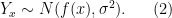
But if we specify ${y}$ , then things get a lot more interesting: if ${f}$ is not invertible, then the most we can say about ${X_y}$ is that

$\displaystyle X_y \in f^{-1}\left(y + Z\right), \qquad Z \sim N(0,\sigma^2) \ \ \ \ \ (3)$

or that ${X_y}$ is somewhere in the preimage, under ${f}$ , of a Gaussian random variable with mean ${y}$ and variance ${\sigma^2}$ . Unless we are in an exceptional situation (e.g., if ${f}$ is one-to-one), it is reasonable to say that (3) expresses a “more complex” statement compared to (2). From this viewpoint, it is more reasonable to say that ${x}$ is the input that causes ${y}$ , and not the other way around. (This way of thinking about causality has, in fact, already found its way into machine learning literature.) The paper of Willems contains a lot more insightful examples and thought-provoking discussion.

So, to summarize: the misunderstanding about conditioning that Larry Wasserman has sought to clear up persists not only in statistics, but also in all other fields involving stochastic systems, such as communications, control, machine learning, etc., and we should always be careful not to fall into this trap.

M	T	W	T	F	S	S
				1	2	3
4	5	6	7	8	9	10
11	12	13	14	15	16	17
18	19	20	21	22	23	24
25	26	27	28	29	30	31

Stochastic kernels vs. conditional probability distributions

One thought on “Stochastic kernels vs. conditional probability distributions”

Leave a comment Cancel reply

Share this:

Related

One thought on “Stochastic kernels vs. conditional probability distributions”

Leave a comment Cancel reply